I am working on using a Bayesian model to estimate parameters for our reward learning data. I’m extending Nate Haines’ Double Update Model for Reversal Learning (Ahn, Haines, and Zhang 2017). Nate modified the version available in his package hBayesDM to work with our dataset, which is a deterministic Reversal Learning task. I have since incrementally extended it to handle two different tasks (reward and punishment learning) and repeated runs.
In the latest, repeated runs version, double_update_rpo_repeated_runs, I am getting values that are quite different to earlier versions. There two possible explanations I have for this:
- Either the former or current model isn’t well designed. One or the other isn’t reliable. The difference between the two is consistently inconsistent. We need to work out which is mis-specified.
- Variational Bayes gives us different results each time we run the same model. Variational Bayes is known to be less precise (but faster) than Monte Carlo Markov Chain estimation (Blei, Kucukelbir, and McAuliffe 2017).
These need to be tested out! So what we need to do is:
- run the models twice each
- save values
- compare Run1 mu, alpha, beta values for G2RiskyNoMeth and G3RiskyMeth
Method
The hard part is running the model! This is done here. Let’s compare:
double_update_rpo_repeated_runs.stan, the latest model designed for multiple runsdouble_update_rp_erroneous.stan, processes reward and punishment data but only one run; there was an error that confused reward inverse temperature variance with punishment learning rate variance; I’ve included that here so we can compare to the resutls we obtained before the error was discovered.double_update_rp_fixed.stan, as above, but with the error fixed.double_update.stan, Processes only reward or punishment data.
We also want to run several times.
models_to_run<-c("double_update_rpo_repeated_runs","double_update_rp_fixed","double_update_rp_erroneous","double_update")
times_to_run=3
The run-wrapper now takes a “file suffix” which means we can run it multiple times, each time with a different suffix, and the run will be saved and given an appropriate name.
As we run these we need to be careful not to use up too much memory. We probably ought to extract just the values we need, which would exclude the individual subject values, then take each object out of memory.
if(file.exists("model-summaries.RData")){
  load(file="model-summaries.RData")
}else{
  model.summaries <- vector("list", 2*length(models_to_run)*times_to_run)
}

if(any(sapply(model.summaries,is.null))){
  for (g in 2:3){
    for (m in models_to_run){
      for (t in 1:times_to_run){
        print (paste0(g,m,t,collapse=", "))
        #only run reward and punishment when we can
        if(models_to_run %in% c("double_update_rpo_repeated_runs","double_update_rp_fixed","double_update_rp_erroneous")){
          rp<-c(1,2)
        }else{
          rp<-c(2)
        }
        #only run multiple runs when we can
        if(models_to_run %in% c("double_update_rpo_repeated_runs")){
          runs=c(1,2)
          generatePosteriorTrialPredictions=FALSE
        }else{
          runs=c(1)
          generatePosteriorTrialPredictions=NA
        }
        #run the model
        fit<-lookupOrRunFit(
          run=runs,groups_to_fit=g, model_to_use=m,includeSubjGroup = FALSE,
          rp=rp,
          model_rp_separately=TRUE,model_runs_separately = TRUE, include_pain=FALSE,
          fileSuffix=paste0("20170923_test_iteration_",as.character(t),generatePosteriorTrialPredictions=generatePosteriorTrialPredictions)
          )

        cat("...model loaded. Extracting...")
        #save just the output we want.
        first_empty_list_pos<-min(which(sapply(model.summaries,is.null)))
        print(paste("first_empty_list_pos is", as.character(first_empty_list_pos)))


        if(m=="double_update_rpo_repeated_runs"){
          model.summaries[[first_empty_list_pos]]<-
                      list("summaryObj"=data_summarize_double_update_rpo_repeated_runs(rstan::extract(fit$fit)),
                           "g"=g,"m"=m,"t"=t)
        }else if(m=="double_update_rp_erroneous" || m=="double_update_rp_fixed"){
          model.summaries[[first_empty_list_pos]]<-
                      list("summaryObj"=data_summarize_double_update_rp(rstan::extract(fit$fit),
                                                                      run = runs),
                           "g"=g,"m"=m,"t"=t)
        }else if(m=="double_update"){
          model.summaries[[first_empty_list_pos]]<-
                      list("summaryObj"=data_summarize_double_update(rstan::extract(fit$fit),
                                                                     outcome.type = rp,
                                                                     run = runs),
                           "g"=g,"m"=m,"t"=t)
        }else{
          stop("f^<%! I don't recognize that model.")
        }
        #remove the fit object from memory, because it is pretty large!
        rm(fit)
        print("...summary data extracted.")
      }
    }
  }
  save(model.summaries,file="model-summaries.RData")
}
Results
For each of the four models, we can compare to see how closely analyses runs matched one another. For each of the Run1 mu, sigma, alpha, beta values for G2RiskyNoMeth and G3RiskyMeth, we can see how much variance exists within and how much variance exists between models.
#arrange all the data into a single data table.
model.summary.all<-NULL
for(ms in model.summaries){
  ms.summaryObj<-ms$summaryObj
  ms.summaryObj$Group<-ms$g
  ms.summaryObj$ModelName<-ms$m
  ms.summaryObj$AnalysisRepetition<-ms$t
  if(is.null(model.summary.all)){
    model.summary.all<-ms.summaryObj
  }else{
    model.summary.all<-rbind(model.summary.all,ms.summaryObj)
  }
}
Alpha mu (learning rate)
##                               Df Sum Sq Mean Sq  F value   Pr(>F)
## factor(AnalysisRepetition)     2  0.094   0.047    28.32 5.32e-13 ***
## factor(Group)                  1 26.309  26.309 15902.67  < 2e-16 ***
## ModelName                      3  2.508   0.836   505.33  < 2e-16 ***
## Residuals                  14963 24.754   0.002
## ---
## Signif. codes:  0 '***' 0.001 '**' 0.01 '*' 0.05 '.' 0.1 ' ' 1
## Single term deletions
##
## Model:
## Value ~ factor(AnalysisRepetition) + factor(Group) + ModelName
## Df Sum of Sq RSS AIC F value Pr(>F)
## <none> 24.754 -95866
## factor(AnalysisRepetition) 2 0.0937 24.848 -95813 28.316 5.321e-13
## factor(Group) 1 26.3088 51.063 -85029 15902.675 < 2.2e-16
## ModelName 3 2.5080 27.262 -94427 505.327 < 2.2e-16
##
## <none>
## factor(AnalysisRepetition) ***
## factor(Group) ***
## ModelName ***
## ---
## Signif. codes: 0 '***' 0.001 '**' 0.01 '*' 0.05 '.' 0.1 ' ' 1It appears that repetition did make a difference, but most of the variance here really does seem to be in the model name (and even more between groups!)
Beta mu (inverse temperature)
##                               Df Sum Sq Mean Sq F value Pr(>F)
## factor(AnalysisRepetition)     2   2.41    1.21   195.7 <2e-16 ***
## factor(Group)                  1  57.86   57.86  9390.1 <2e-16 ***
## ModelName                      3   7.80    2.60   422.1 <2e-16 ***
## Residuals                  14963  92.19    0.01
## ---
## Signif. codes:  0 '***' 0.001 '**' 0.01 '*' 0.05 '.' 0.1 ' ' 1
## Single term deletions
##
## Model:
## Value ~ factor(AnalysisRepetition) + factor(Group) + ModelName
## Df Sum of Sq RSS AIC F value Pr(>F)
## <none> 92.194 -76182
## factor(AnalysisRepetition) 2 2.411 94.605 -75799 195.68 < 2.2e-16
## factor(Group) 1 57.856 150.050 -68892 9390.07 < 2.2e-16
## ModelName 3 7.803 99.997 -74972 422.14 < 2.2e-16
##
## <none>
## factor(AnalysisRepetition) ***
## factor(Group) ***
## ModelName ***
## ---
## Signif. codes: 0 '***' 0.001 '**' 0.01 '*' 0.05 '.' 0.1 ' ' 1We can visualize how that looks.
source("visualization/geom_hdi.R")

m.reward.mu.run1<-model.summary.all[Motivation=="Reward" & Statistic=="mu" & Run==1]
#table(m.reward.mu.run1$ModelName)
#for clarity's sake...
m.reward.mu.run1$ModelName<-sub("double_update","DU",m.reward.mu.run1$ModelName)

  #plotly::ggplotly(p)
  ggplot(m.reward.mu.run1[Parameter=="alpha"],aes(x=Value,fill=factor(Group),color=factor(Group)))+
    geom_freqpoly(alpha=0.9,binwidth=0.001)+
     geom_hdi(size=2, lineend = "round",alpha=0.5,credible_mass=0.95)+
    facet_grid(ModelName~AnalysisRepetition)+
    labs(title=paste0("mu statistic in reward rounds, alpha"))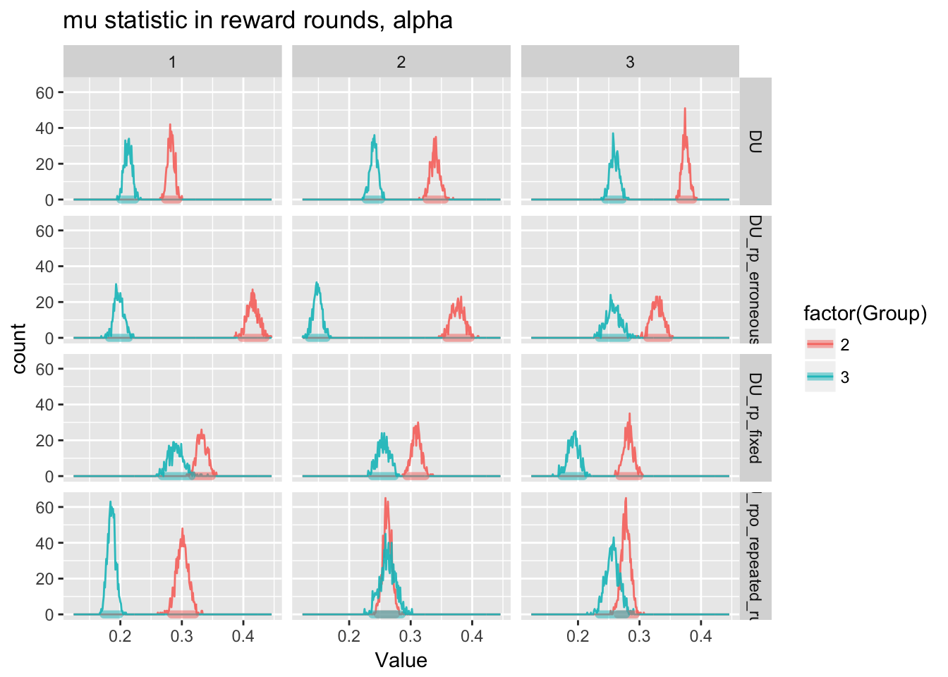
  ggplot(m.reward.mu.run1[Parameter=="beta"],aes(x=Value,fill=factor(Group),color=factor(Group)))+
    geom_freqpoly(alpha=0.9,binwidth=0.001)+
     geom_hdi(size=2, lineend = "round",alpha=0.9,credible_mass=0.95)+
    facet_grid(ModelName~AnalysisRepetition)+
    labs(title=paste0("mu statistic in reward rounds, beta"))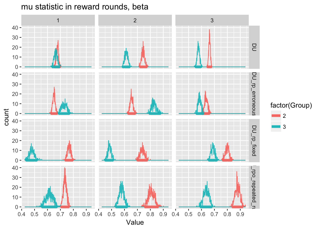
There is one thing consistent across all samples for the reward round, no matter what model is used and across both repetitions. Meth users have lower or similar learning rates compared to Non-users. In no runs did we find that meth users had higher learning rates or inverse temperatures than non-users.
However, there is considerable variation across both runs and models. Importantly, for the final model, which takes into account Run2 and also calculates both reward and punishment, posterior alpha (learning rate) samples overlapped such that it is visually not clear there was a significant difference between groups. If we examine the difference between groups for each analysis, we can see that the 95% HDI includes (and in fact, is pretty closely centered around) zero for two of the three analyses run for the final model.
alpha_lastModel<-tidyr::spread(m.reward.mu.run1[Parameter=="alpha" & ModelName=="DU_rpo_repeated_runs"],
              Group, Value)

alpha_lastModel$GroupDifference<-alpha_lastModel$`2`-alpha_lastModel$`3`

plotly::ggplotly(ggplot(alpha_lastModel,
         aes(x=GroupDifference,color=factor(AnalysisRepetition)))+
    geom_freqpoly(alpha=0.9,binwidth=0.001)+
     geom_hdi(size=2, lineend = "round",alpha=0.5,credible_mass=0.95)+
    labs(title=paste0("learning rate NoMeth-Meth group difference credible values, by Analysis\nWith 95% Highest Density Intervals")))
Differences between the groups varied considerably depending on whether we examine Analysis Run 1 or Run 2. For the second analysis, there were very small differences between groups; for the first analysis differences seemed to be larger. There was also quite a lot of variation between the parameters estimated by the different models, although it is not clear that it is necessary to go to the model used to explain the difference - this may simply be due to the random effects of each analysis.
Discussion
\(\beta\) values are reasonably consistent between repeated trials. But for our final and most comprehensive analysis, variational bayes varies widely between concluding that there is a real between-group difference and that there is not.
Thus, to really get at a decent answer we will want to take a look at using an MCMC estimator.
References
Ahn, Woo-Young, Nathaniel Haines, and Lei Zhang. 2017. “Revealing Neurocomputational Mechanisms of Reinforcement Learning and Decision-Making with the HBayesDM Package.” Computational Psychiatry. MIT Press.
Blei, David M, Alp Kucukelbir, and Jon D McAuliffe. 2017. “Variational Inference: A Review for Statisticians.” Journal of the American Statistical Association, no. just-accepted. Taylor & Francis.